Read data

This tutorial jupyter notebook and the sample.npz it uses can be found at https://github.com/timpyrkov/mhealthdata/tree/master/docs/notebook.

Many smartphone health apps have their own data format.

mHealthData is a tool to load to pandas Dataframes all basic health data (steps, sleep, bpm, rhr, and weight) from different formats (.csv, .json, .xml stored in various sub-folders as well as equispaced or with arbitrary timestamps for start and end).

The code cell below is an example. It will only run if you provide a valid path to a health data export and replace FitbitLoader() with ShealthLoader() for Samsung Health export or HealthkitLoader() for Apple Healthkit export.

Tutorial does not include a raw data export. If you have one, please uncomment the commented lines in two cells below and run the piece of code to read data. Tutorial provides a randomly generated sample.npz to show examples of data analysis and visualization after it were read and converted to NumPy arrays.

import mhealthdata

# path = '/Users/username/Downloads/wearable_data/User/'
# wdata = mhealthdata.FitbitLoader(path)

# """ Show userdata """
# print(wdata.userdata)

# """ Show loaded devices """

# print(wdata.devices)

# """ Show lodaded dataframes """
# print(wdata.dataframes)

# """ Show 'steps' dataframe """
# print(wdata.df['steps'].head())

Data to NumPy

Device key all is default. You may want to gete data separately for wearable or mobile, or even for iPhone or Apple Watch if those were found.

get_device_data() method converts data for specific wearable or mobile device to a dictionary of NumPy arrays.

save_device_npz() method saves data for specific wearable or mobile device to .npz files for furthur use e.g. in another notebook (the .npz file is less then 25Mb for a 2-year sample).

A saved data sample can be loaded using NumPy.

# """ Get data for 'all' devices """
# data = wdata.get_device_data('all')

# """ Or save data to an .npz file """
# wdata.save_device_npz('all')

import numpy as np

""" Open a saved 'sample.npz' """
data = np.load('sample.npz')

""" List loaded NumPy arrays """
for key in data:
    print(key, data[key].shape, data[key].dtype)

idate (28,) int64
steps (28, 1440) float64
sleep (28, 1440) float64
bpm (28, 1440) float64
rhr (28,) float64
weight (28,) float64

Date and time

Date is stored as idate is ordinal date - number of days since January 1st of year 1.

Time is given in the number of minutes since midnight 0 - 1440 as the index along the second axis for 2D arrays (steps, sleep, bpm).

Datetime python lib modules datetime and timedelta can be used to convert idate to human-readable date-time format.

from datetime import datetime, timedelta

idates = data['idate'] # ordinal days (January 1st of year 1 - is day 1)
dates = [datetime.fromordinal(d) for d in idates]
print(f'Date range {dates[0]} - {dates[-1]}')

Date range 2021-02-01 00:00:00 - 2021-02-28 00:00:00

Visualization

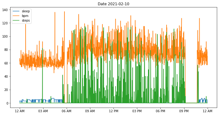
Intraday data visualiztion is simple.

For bpm we observe gaps in data when bpm drops to zero when a user took off their wristband.

For steps zero values indicate both missing data and not-walking, e.g. during sleep.

For sleep zero values indicate not sleeping.

import pylab as plt

i = 9 # Day 10 has index 9
plt.figure(figsize=(12,6), facecolor='white')
plt.title(f'Date {dates[i].strftime("%Y-%m-%d")}')
for dname in ['sleep', 'bpm', 'steps']:
        plt.plot(data[dname][i], label=dname)
mhealthdata.xticks_hours(dt=3, mode="12h")
plt.legend()
plt.show()

Sleep duration

Bouts of sleep bouts are often split between two days.

Utility fiunction find_nonzero_intervals() returns list of indices of start and end of a continuous non-zero range (e.g. sleep bout) along the flattened sleep array.

sleep = data['sleep'].flatten()
bouts = mhealthdata.find_intervals(sleep)
duration = [bout[1] - bout[0] for bout in bouts]
print('Sleep duration [minutes]:', duration)

Sleep duration [minutes]: [360, 410, 428, 398, 421, 450, 426, 457, 406, 431, 393, 479, 434, 306, 156, 399, 475, 420, 379, 406, 369, 292, 155, 416, 128, 299, 401, 325, 315, 116]

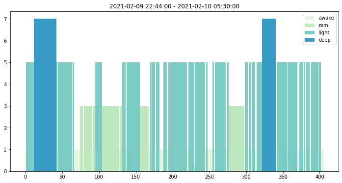
Sleep stages

Utility fiunction sleep_stage_dict() returns dictionary to decode numerically-coded sleep stages.

Let us plot sleep stages for a sleep bout between Feb 9th and 10th.

j0, j1 = bouts[8] # Day 9 has index 8
x = sleep[j0:j1]
t = np.arange(len(x))

date_time_start = dates[j0 // 1440] + timedelta(minutes = int(j0) % 1440)
date_time_end = dates[j1 // 1440] + timedelta(minutes = int(j1) % 1440)

stages = mhealthdata.sleep_stage_dict()

plt.figure(figsize=(12,6), facecolor='white')
plt.title(f'{date_time_start} - {date_time_end}')
for x_ in np.unique(x):
    mask = x == x_
    label = stages[x_]
    color = plt.cm.GnBu(0.1 * x_)
    plt.bar(t[mask], x[mask], width=1, color=color, label=label)
plt.legend()
plt.show()

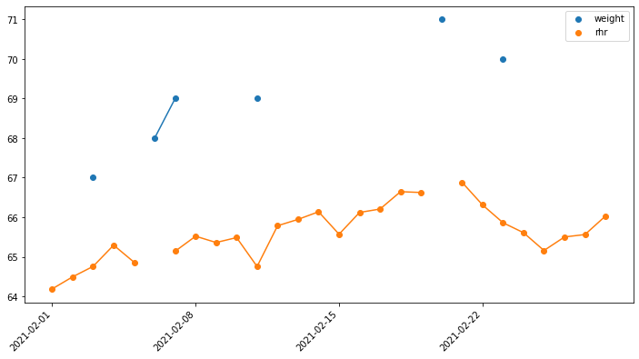
Data correlation

Visual inspection tells us that rhr and weight are correlated.

x = data['weight']
y = data['rhr']
t = data['idate']

""" IMPORTANT: zero values indicate missing data and should be disregarded """
x[x == 0] = np.nan
y[y == 0] = np.nan

plt.figure(figsize=(12,6), facecolor='white')

plt.plot(t, x) # plot lines
plt.scatter(t, x, label='weight') # plot dots

plt.plot(t, y) # plot lines
plt.scatter(t, y, label='rhr') # plot dots
mhealthdata.xticks_dates(t, "week")

plt.legend()
plt.show()

Data interpolation

Missing data reduce the number of overlapping data-points. Technically low number of data-points results in correlation coefficient r with poor statistical significance p-value ~ 0.25. Statistically significant result shoud have p-value < 0.05.

We will use interpolation data to fill the gaps and improve the statistical significance.

A study Pyrkov T.V. et al., Nature Communications 12, 2765 (2021) shows high consistency of recovery rates in quite different biological signals - physical activity measured by consumer wearable devices and laboratory blood cell counts. The typical recovery time of 1-2 weeks. The finding suggests it may be safe to use averaging windows or impute data gaps of several day length (though both affect noise and correlation and therefore should be used with caution).

from scipy.stats import pearsonr

x = data['rhr']
y = data['weight']
t = data['idate']

""" IMPORTANT: zero values indicate missing data and should be disregarded """
mask = (x > 0) & (y > 0)
r, p = pearsonr(x[mask], y[mask])
print(f'Correlation {r:.2f}, P-value {p:.2g}')

""" Interpolate rhr data """
mask = (x > 0)
x_ = np.interp(t, t[mask], x[mask])
print('\nMissing RHR data imputed with linear interpolation\n')

mask = (x_ > 0) & (y > 0)
r, p = pearsonr(x_[mask], y[mask])
print(f'Correlation {r:.2f}, P-value {p:.2g}')

Correlation 0.75, P-value 0.25

Missing RHR data imputed with linear interpolation

Correlation 0.87, P-value 0.024